On the difficulty of training Recurrent Neural Networks
Literature url
The author’s motivation
- In this paper we attempt to improve the understanding of the underlying issues by exploring these problems from an analytical, a geometric and a dynamical systems perspective.
RNN’s features
- with the distinction that we allow connections among hidden units associated with a time delay
- Through these connections the model can retain information about the past inputs, enabling it to discover temporal correlations between events that are possibly far away from each other in the data (a crucial property for proper learning of time series).
- Problem: While in principle the recurrent network is a simple and powerful model, in practice, it is unfortunately hard to train properly. Among the main reasons why this model is so unwieldy are the vanishing gradient and exploding gradient problems described in Bengio et al.
RNN model - some key points
-
RNN里面代价函数
A cost $\varepsilon$ measures the performance of the network on some given task and it can be broken apart into individual costs for each step $\varepsilon=\sum_{1 \leq t \leq T} \varepsilon_{t}$, where $\varepsilon=L(X_t)$ .
RNN里面代价函数是每个时刻的代价或者的损失的求和。
Exploding and Vanishing Gradients
- As introduced in Bengio et al. (1994), the exploding gradients problem refers to the large increase in the norm of the gradient during training. Such events are caused by the explosion of the long term components, which can grow exponentially more then short term ones. The vanishing gradients problem refers to the opposite behaviour, when long term components go exponentially fast to norm 0, making it impossible for the model to learn correlation between temporally distant events.
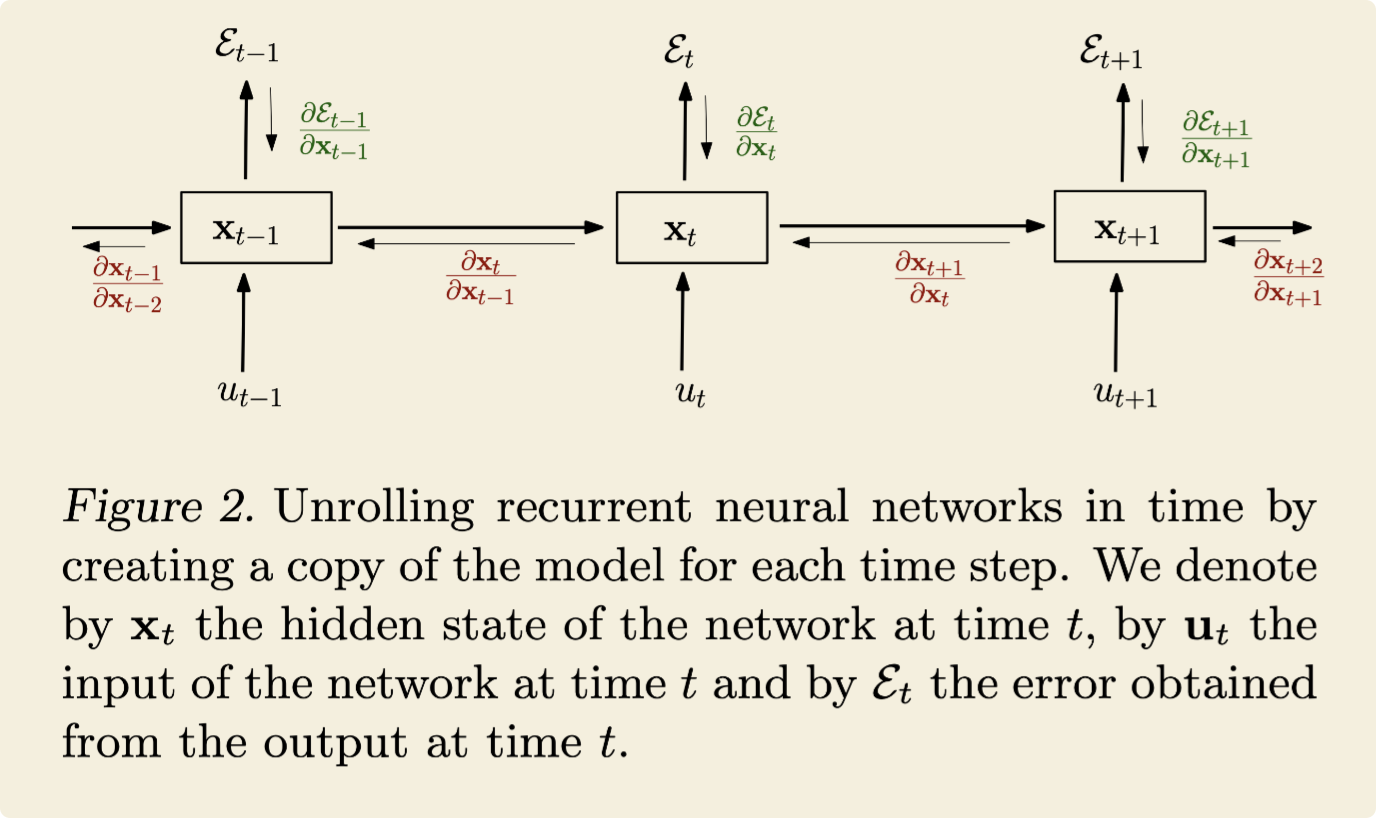
Backpropagation Through Time (BPTT)
- RNN Formula
formula(1): A generic recurrent neural network, with input $u_t$ and state $x_t$ for time step $t$.
formula(2): The specific parametrization, in order to provide more precise conditions and intuitions about the everyday use-case.
The parameters of the model are given by the recurrent weight matrix $W_{rec}$, the biases $b$ and input weight matrix $W_{in}$, collected in $\theta$ for the general case. $x_0$ is provided by the user, set to zero or learned, and $\theta$ is an element-wise function (usually the tanh or sigmoid )
A cost $\varepsilon$ measures the performance of the network on some given task and it can be broken apart into individual costs for each step $\varepsilon=\sum_{1 \leq t \leq T}\varepsilon_t$ , where $\varepsilon_t=L(x_t)$. 代价函数可以拆分成每个时间步上的代价函数.
- where the recurrent model is represented as a deep multi-layer one (with an unbounded number of layers ) and backpropagation is applied on the unrolled model .
The geometrical interpretation
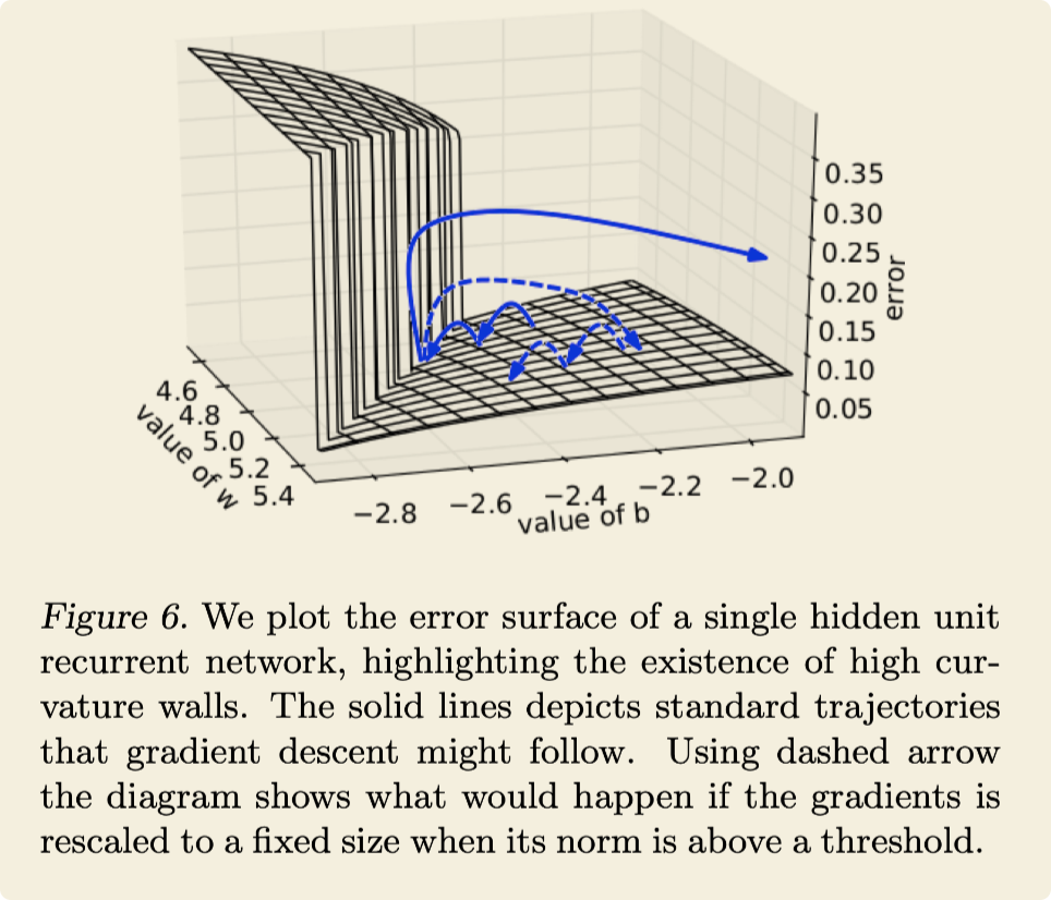
- when stochastic gradient descent (SGD) reaches the wall and does a gradient descent step, it will be forced to jump across the valley moving perpendicular to the steep walls, possibly leaving the valley and disrupting the learning process. 如果随机梯度下降的话,在到达悬崖边上,梯度会变得特别大,可能会以一个很大的步伐去远离那个山谷,就像图中的朝右的蓝色实线一样,这样会导致打断“学习”过程,寻找不到局部最优。